Dropdown menus are commonly used for error prevention, input validation, or restricting selections in single-choice questions. In multilevel cascading forms, such as selecting “Taipei City” in the first level and then choosing one of its 12 districts in the second level, this tutorial will also share a method for automatic color display.
Creating Dropdown Menu Items in Excel
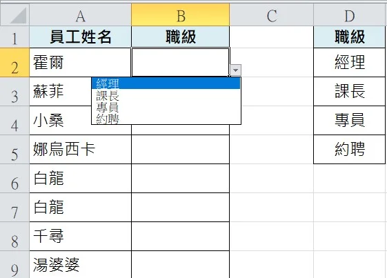
List out the items to be selected in the menu. They can be listed vertically, horizontally, or as real-time function computation results, such as using the COUNT function. However, they must be within the same file to work.

Setting up the Menu
After selecting the cells where the menu will be added, go to the top toolbar > Data > Data Validation > Settings. In the cell, allow a list, and then click the small data selection button on the right side of the Source box. Choose the menu items that were previously created, and it is recommended to check the “Ignore blank” option. The prompt message can display explanations when the dropdown menu is selected but is not commonly used.


Multilevel Cascading Dropdown Menus
For example, if I want to select the colleagues’ residential city and district, it wouldn’t make sense to select “Taipei City” and have all the districts in Taiwan available for selection. In this case, a two-level cascading menu is needed, which requires slightly more complex settings.
Creating Items for the Two-level Menu: Defining Names
List the first-level items and their corresponding second-level items, such as “Taipei City” and its districts like Shilin, Beitou, Wenshan, etc., as shown in the picture. Then go to the top toolbar > Formulas > Define Name. Select a name, such as “City,” and refer to all the districts in the box. Make sure to define a name for each row.

Afterward, you can confirm in Formulas > Name Manager.
Creating the First-Level Menu
Assuming we want to create the first level in cell B2, go to the top toolbar > Data > Data Validation > Settings. Select “List” and choose the two cities that were created earlier as the source.

Creating the Second-Level Menu
Assuming we want to create the second level in cell C2, go to the top toolbar > Data > Data Validation > Settings. Select “List” and enter the function “=INDIRECT(B2)” as the source. That’s it! For creating the third, fourth levels, etc., assume we want to create them in cell C2. Follow the same steps as above, and for more levels, continue with this method. Excel may default to “=INDIRECT($B$2)” for subsequent levels, which is also fine.
If you see an error while evaluating the formula, it is because the city is empty. Just proceed boldly, and you will be able to use the two-level cascading dropdown menu successfully.
Editing Colors
This is essentially setting up rules. After selecting the area where you want to edit colors, go to the top toolbar > Home > Conditional Formatting > New Rule.
Choose “Format only cells that contain” and set the cell value equal to “Shilin District” (or any other condition), then click “Format.”
Here, you can set fill color, change font size, apply borders, etc., when the cell value is “Shilin District.” Afterward, you have successfully completed the task.

In addition to dropdown menus, you can click here to see more Excel tutorials. Due to the large amount of content, please refer to Microsoft’s instructions on inserting multiple selection menus for information on multi-select menus.